Contour Lines: A V Pointing Uphill Marks a Stream Valley
The Reading Room Published
Short answer
On a topographic map, brown contour lines usually bend into V-shaped points where a blue stream crosses them. Each point aims upstream, toward higher ground, because the line runs back up the valley.
Viewing card
- Where
- Cascade Range, Washington; corners of the lead map's frame 47.773°–47.797° N, 121.315°–121.365° W
- Seen from
- Map view from above: USGS 3DEP 1/3 arc-second DEM, contoured every 40 m (this page's calculation from the elevation model, not a field survey)
- Captured
- USGS 1/3 Arc Second n48w122 20250813 (publicationDate 2025-08-13); read 2026-11-16 (data version, not a survey date)
- Reading altitude
- In an image: 10.3 m elevation grid, 40 m interval; the V valley is approximately 360 m deep on its north-northeast side and 230 m on its south-southwest side, so it crosses several lines; a rise under 40 m can fall between two lines
- Written by
- The shape of the valley in the elevation model; contours run back up a valley (the V is this page's shorthand, not the manual's word)
This card as data (CSV) About this file
Data: Data available from U.S. Geological Survey, National Geospatial Program.; USGS Professional Paper 60 (1908), public domain
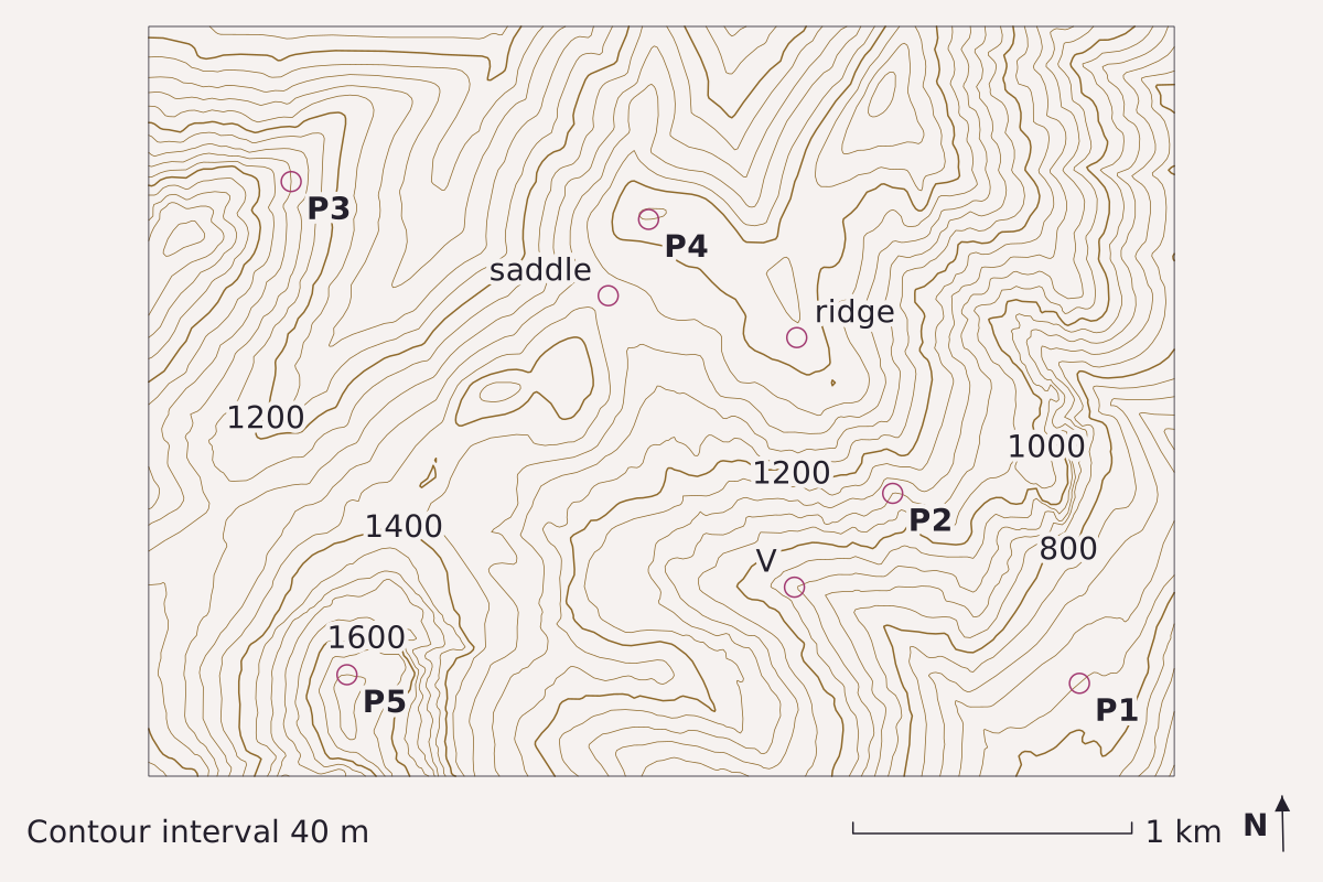
Contours every 40 m for a block of the Cascade Range near 47.79° N, 121.34° W. At V the lines cross a stream valley and point west, up the valley; at the ridge the bends point downhill; the saddle is the low spot on the crest between two summits. North is up, with the map grid about 1.2° off true north. Elevation: USGS 3DEP 1/3 arc-second, n48w122 2025-08-13.
Benchmark Contours from USGS 3DEP 1/3 arc-second DEM; interval 40 m; 5 points checked against the DEM; map corners recomputed from the DEM's georeferencing.
"Contours of a Cascade Range block at a 40 m interval, with five check points" by Meridian & Moraine, https://meridianandmoraine.com/contours/contour-lines/, licensed under CC BY 4.0 (https://creativecommons.org/licenses/by/4.0/).
Data: Data available from U.S. Geological Survey, National Geospatial Program.
The rule is more than a century old. USGS Professional Paper 60, The Interpretation of Topographic Maps by Rollin Salisbury and Wallace Atwood (1908), says a contour line “runs back up the valleys and forward around the points of hills and spurs” (p. 11). The letter V is this page’s shorthand for that bend, not the manual’s own word, and the five points labeled P1 to P5 are listed in the table near the end of the page.
Look at the label V on the map above. According to the elevation model, the valley floor there lies at about 920 m. Within 600 m across the valley, the ground rises to about 1,280 m on the north-northeast side and about 1,150 m on the south-southwest side. Every line that crosses the valley turns west, up the valley, before it swings back out along the far wall.
What is a contour line?
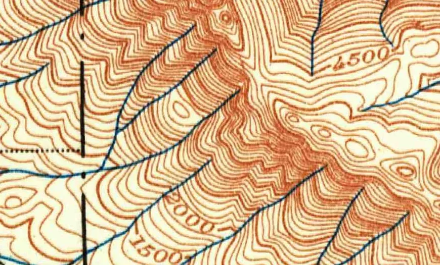
Part of the 1902 USGS topographic sheet for Skykomish, Washington, near Baring: brown contours labeled in feet, such as 1500, 2000 and 4500, crowd onto steep slopes and bend into points where the blue streams cross them.
"Skykomish, Washington, topographic sheet (detail near Baring), 1902" by U.S. Geological Survey — https://commons.wikimedia.org/wiki/File:1902_USGS_topo_map_of_Baring,_Washington.jpg — Public domain (US: U.S. Government work (17 U.S.C. §105), USGS topographic sheet published 1902; EU: published 1902 by a U.S. federal agency, more than 70 years ago); modified: cropped
A contour line connects points of equal elevation. Professional Paper 60 puts it plainly, “Each contour passes through points which have the same altitude” (p. 11), and then offers a test for anyone walking the ground: a person following a contour “will go neither uphill nor downhill, but on a level.”
The current USGS reference sheet Topographic Map Symbols puts the same idea in one line: “Each contour is a line of equal elevation; therefore, contours never cross.” On USGS maps the contours are printed in brown, in lines of different widths.
The 1908 manual also suggests a mental picture. The seacoast is itself a contour, the line of zero elevation, and a line drawn 20 feet above sea level marks where the coast would be “if the sea were to rise or the land to sink 20 feet” (p. 11). Any contour on a map can be imagined the same way, as the shoreline of a sea that is not actually there.
That picture explains the historical sheet above, where each brown line traces a level shoreline around the mountains near Baring. Wherever a blue stream has cut into a slope, the imaginary shoreline must follow the valley inland before it can return along the other side.
Why do contours bend into a V at a stream?
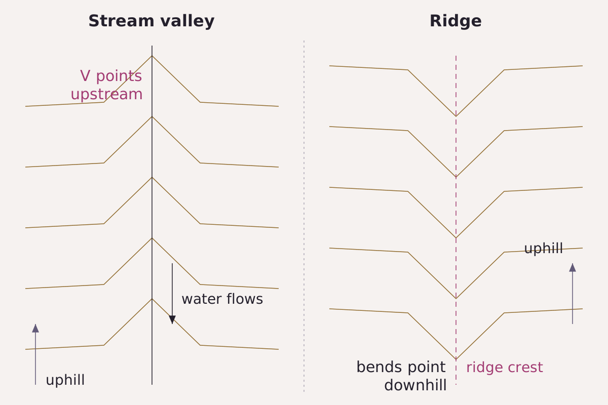
Two kinds of bend, side by side: across a stream valley the points aim upstream, toward higher ground; along a ridge they aim downhill.
Benchmark Schematic, not to scale; bend direction from USGS Professional Paper 60 (1908), p. 11.
"Contour bends at a stream valley and at a ridge, schematic" by Meridian & Moraine, https://meridianandmoraine.com/contours/contour-lines/, licensed under CC BY 4.0 (https://creativecommons.org/licenses/by/4.0/).
Data: USGS Professional Paper 60 (1908), public domain
Consider a single contour approaching a valley. The ground slopes down toward the stream from both sides. A line that keeps one elevation must travel up the valley until the rising stream bed reaches that height, then cross the stream and come back along the other side. Seen from above, that detour forms the V, and its point sits on the stream at the farthest upstream position the line reaches.
A river writes its course into the hills, and the contours read like the indentation left by that pen stroke. Physically, running water wears the valley floor down below the ground beside it. Every contour above the floor has to loop around that cut, so the points stack up along the stream, one above another, aimed toward its source.
A ridge or spur does the opposite. The ground there stands higher than the land on either side, so a contour must swing outward around the end of the ridge, and its bend points downhill. The 1908 manual covers both cases in a single sentence, and on the lead map the label “ridge” marks bends of the second kind.
The shape is not invariably a sharp V. USGS Bulletin 788-E (1928), the Survey’s instructions for its own topographers, warns against “the use of sharp or curved stream reentrants where the opposite should be used” (p. 253). A reentrant is the inward bend of a contour, and that wording treats both a sharp point and a curve as shapes it can take; the same page asks that the turning points of contours along steep drainage channels stay aligned with one another.
According to Professional Paper 60, geologic maps are printed on the same kind of topographic base, with colors for rock units laid over the contours (p. 12). The bends read here carry over to how to read a geologic map.
Close together, far apart: reading slope
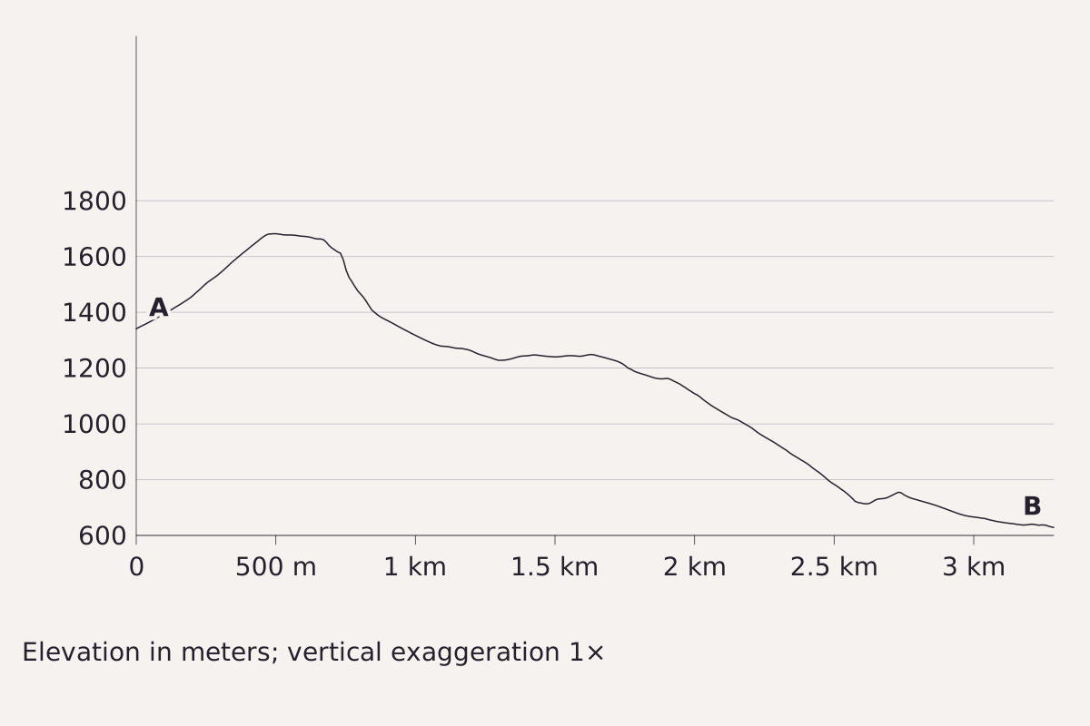
A slice through the same elevation model, from A (47.7765° N, 121.3619° W) to B (47.7759° N, 121.3181° W), about 3.3 km west to east, drawn with no vertical stretch. Where the contours on the map crowd together, the line here drops steeply; where they spread out, it flattens into a bench. Elevation: USGS 3DEP 1/3 arc-second, n48w122 2025-08-13.
Benchmark Profile from USGS 3DEP 1/3 arc-second DEM; vertical exaggeration 1×; 5 points checked against the DEM.
"Elevation profile across the contour map, no vertical exaggeration" by Meridian & Moraine, https://meridianandmoraine.com/contours/contour-lines/, licensed under CC BY 4.0 (https://creativecommons.org/licenses/by/4.0/).
Data: Data available from U.S. Geological Survey, National Geospatial Program.
Spacing shows steepness. In the 1908 manual, contour lines far apart indicate a gentle slope, lines “close together, a steep slope,” and lines that merge into one, “as if each were vertically under the one above it,” indicate a cliff (p. 11). Topographic Map Symbols says the same in modern terms: contours “very close together represent steep slopes,” while widely spaced contours mean relatively level ground.
The profile above turns that rule into a side view. It crosses a summit at about 1,680 m near P5. To the east it drops fast where the contours on the map are tightly packed, levels into a bench near 1,240 m, and then follows a long, steady decline to about 630 m. Because the vertical scale is not exaggerated, every slope appears at its true angle.
A profile makes a selection of its own, too: it records only the single line it follows. A gully 50 m to the side is absent from it. At true vertical scale, small irregularities of a few meters look almost flat.
The cartographer's cut: what the interval hides
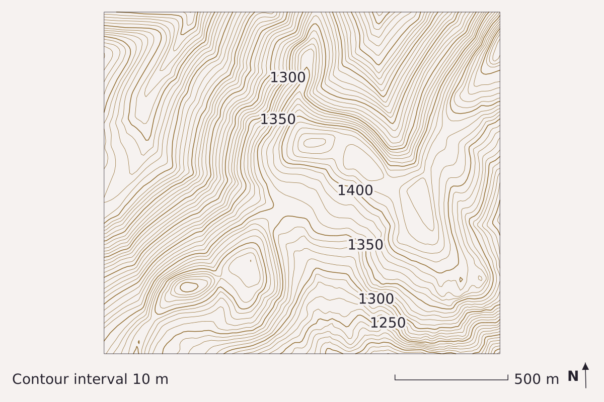
"A ridge top contoured at a 10 m interval" by Meridian & Moraine, https://meridianandmoraine.com/contours/contour-lines/, licensed under CC BY 4.0 (https://creativecommons.org/licenses/by/4.0/).
Data: Data available from U.S. Geological Survey, National Geospatial Program.
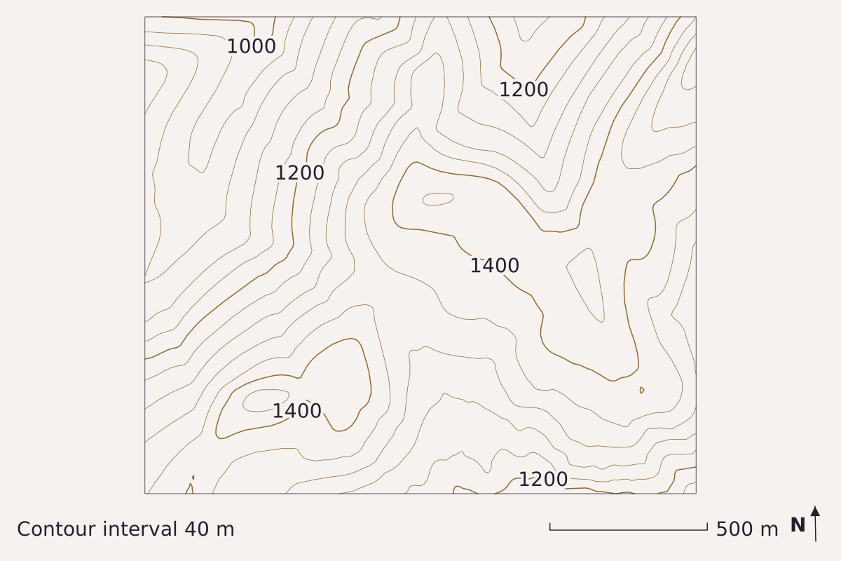
"The same ridge top contoured at a 40 m interval" by Meridian & Moraine, https://meridianandmoraine.com/contours/contour-lines/, licensed under CC BY 4.0 (https://creativecommons.org/licenses/by/4.0/).
Data: Data available from U.S. Geological Survey, National Geospatial Program.
The same ground drawn twice from the same elevation model, first every 10 m, then every 40 m. Some knolls ringed by closed 10 m lines leave no ring at all at 40 m; the larger rises keep only a single small loop. North is up, with the map grid about 1.2° off true north. Elevation: USGS 3DEP 1/3 arc-second, n48w122 2025-08-13.
Benchmark Contours from USGS 3DEP 1/3 arc-second DEM; intervals 10 m and 40 m; 5 points per map checked against the DEM; map corners recomputed from the DEM's georeferencing.
Every map leaves things out to stay readable. Meridian & Moraine calls that omission the cartographer's cut: whatever a map leaves out, merges or bends so that it can be read at all. On a contour map, the most important cut is the contour interval, the vertical distance between one line and the next.
The pair above shows that cut at work. At a 10 m interval, several small knolls on this ridge top carry their own closed rings, whereas at 40 m a knoll 30 m high can fall entirely between two lines and leave no trace. The ground is identical in both maps. Only the interval has changed.
Mapmakers choose the interval to suit the terrain. Professional Paper 60 reports that it may be as small as 10 feet in flat country and 200 feet in a mountainous region, and that it is stated at the bottom of each map (p. 12). Topographic Map Symbols gives 10 feet or less for a relatively flat area and 100 feet or more in mountainous areas, with the interval printed in the margin of each USGS map.
The 1928 instructions describe a second, deliberate kind of cut. Bulletin 788-E permits a field topographer to adjust a contour slightly to “bring out prominent and characteristic relief,” disregarding a measured elevation by “as much as 10, 20, or even 30 per cent of the contour interval” where the interval is large and the scale small (p. 253). On a hand-drawn sheet, then, a line can depart a little from its exact elevation on purpose.
The maps on this page are computed rather than sketched, so their cut is different. The five check points agree with the elevation model to within 0.26 m. That figure measures how closely the drawn lines follow the model, not how closely the model matches the ground, and the 10.3 m grid the maps are computed on already spreads any cliff across at least one grid cell.
Index contours and the numbers on the lines
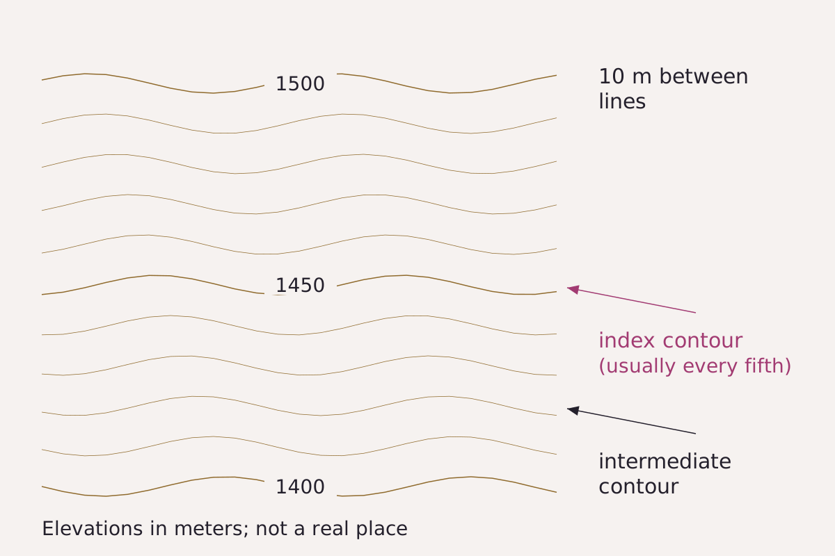
Index and intermediate contours on a made-up slope at a 10 m interval: the wider lines carry the numbers, and the four narrower lines between each pair fill in the shape.
Benchmark Schematic, not to scale; line weights from USGS Topographic Map Symbols and the every-fifth-line rule from Professional Paper 60 (1908).
"Index and intermediate contours, schematic" by Meridian & Moraine, https://meridianandmoraine.com/contours/contour-lines/, licensed under CC BY 4.0 (https://creativecommons.org/licenses/by/4.0/).
Data: USGS Topographic Map Symbols and Professional Paper 60, public domain
Not every contour carries a number. Topographic Map Symbols explains that index contours are printed wider, with elevation values repeated at several places along them, while the narrower intermediate and supplementary contours between them “help to show more details of the land surface shape.”
Professional Paper 60 describes the spacing of the numbered lines: certain contours, “usually every fifth one,” are emphasized and labeled with their elevation above sea level (p. 12). At a 40 m interval, that puts an index line every 200 m. The lead map follows the pattern. Its wider lines are labeled 800, 1000, 1200, 1400 and 1600.
To find the height of an unlabeled line, start at the nearest index contour and count outward, one interval per line. The direction of the nearest stream shows which way is down. On the 10 m map in the pair above, the wider lines carry labels every 50 m.
Contour lines are only one way to draw a mountain. Shaded relief shows the same kind of terrain with light and shadow instead, and it makes its own choices about what to emphasize.
The contours that helped weigh the Earth
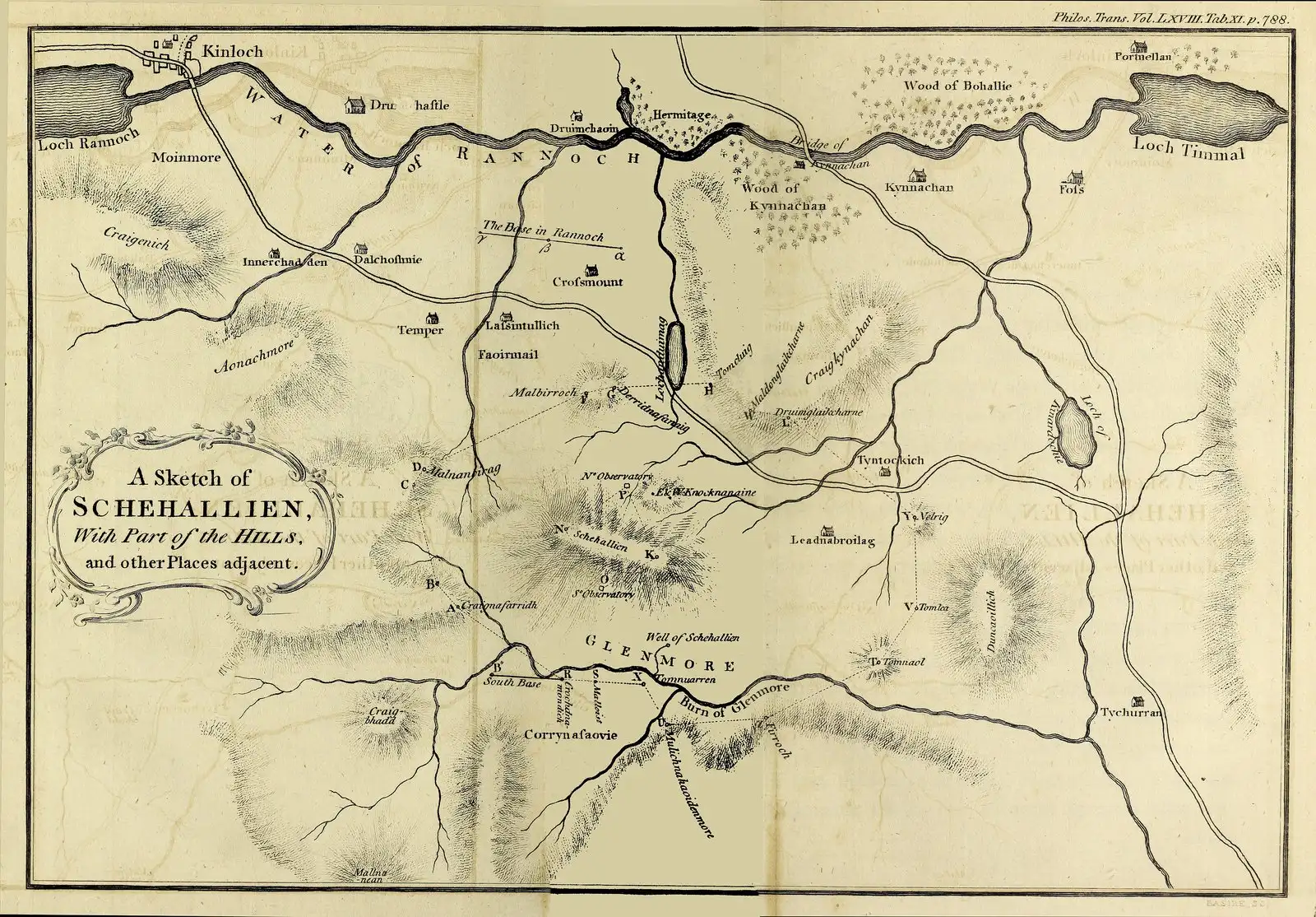
The plate of Schehallien and the country around it printed with the 1778 calculations, Tab. XI in volume 68 of Philosophical Transactions, with the north and south observatories marked on the hill. The hills on this published sketch are shaded; the level lines described on pages 756–757 were drawn on working plans.
“A Sketch of Schehallien, with Part of the Hills, and other Places adjacent, from An Account of the Calculations made from the Survey and Measures taken at Schehallien (Philosophical Transactions 68, Tab. XI)”, Charles Hutton; public domain.
Full credit
"A Sketch of Schehallien, with Part of the Hills, and other Places adjacent, from An Account of the Calculations made from the Survey and Measures taken at Schehallien (Philosophical Transactions 68, Tab. XI)" by Charles Hutton — https://commons.wikimedia.org/wiki/File:Schehallien_Sketch_Hutton_1779.jpg — Public domain (US: published 1779, before 1931; EU: author Charles Hutton died 1823, more than 70 years ago; plate signed Basire sc., engraver's death year not traced); modified: resized
Schiehallion, spelled Schehallien in the eighteenth century, is a mountain in Perthshire, Scotland. In a paper read to the Royal Society on 6 July 1775, the Astronomer Royal, Nevil Maskelyne, reported observations made on the mountain “for finding its Attraction” (Philosophical Transactions 65, p. 500). He had proposed in 1772 to measure the pull of “some hill in this kingdom” by watching the stars.
The experiment compared two independent measurements of the same north–south distance across the mountain. Star observations at an observatory on each side produced a difference of latitude of 54.6 seconds of arc, while the ground survey produced only 42.94 seconds. Maskelyne wrote that the difference of 11.6 seconds “is to be attributed to the sum of the two contrary attractions of the hill” (p. 531), meaning the mountain had pulled each observatory’s plumb line toward itself.
Maskelyne concluded that “the mountain Schehallien exerts a sensible attraction” (p. 532). On the same page he wrote that the density of the hill, compared with the Earth’s, could not be properly settled until its shape and size had been worked out from the survey. He called that “a work of much time and labour,” and the results came three years later.
Charles Hutton read his account of the calculations to the Royal Society on 21 May 1778 (Philosophical Transactions 68, p. 689). He is not the same person as James Hutton, the geologist whose interpretation of rock layers appears on the Siccar Point page. Charles Hutton worked from a survey conducted in 1774, 1775 and 1776 under Maskelyne’s direction, and the surveyed points left many small spaces on his plans without any known elevation.
His solution appears on pages 756–757. “This method was the connecting together by a faint line all the points which were of the same relative altitude,” Hutton wrote, producing “a great number of irregular polygons” that “were the figures of so many level or horizontal sections of the hills.” With those lines in place, he could estimate the elevation of each small space, generally to within ten feet and often within five.
How do you read the next contour map?
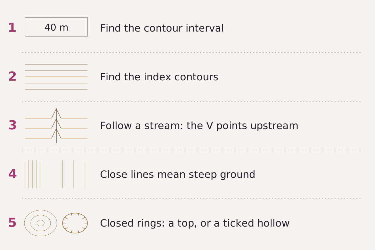
Five checks for any contour map, in the order this page uses them.
Benchmark Schematic, not to scale; steps drawn from USGS Professional Paper 60 (1908) and Topographic Map Symbols.
"Five steps for reading a contour map, schematic" by Meridian & Moraine, https://meridianandmoraine.com/contours/contour-lines/, licensed under CC BY 4.0 (https://creativecommons.org/licenses/by/4.0/).
Data: USGS Professional Paper 60 and Topographic Map Symbols, public domain
The same five checks apply to a historical sheet, a modern USGS map or the lead map on this page:
- Find the contour interval in the margin or along the bottom edge, because a rise smaller than the interval can fall between two lines and leave no trace.
- Find the index contours, the wider numbered lines, and count upward or downward from them.
- Follow a stream to where it crosses the contours, and notice that the points of the bends aim upstream, toward higher ground.
- Compare the spacing, since closely packed lines indicate steep ground and widely spaced lines indicate gentle ground.
- Look inside closed rings. Professional Paper 60 notes that contours surround hollows “just as they surround hills,” and that small hollows are usually marked by short ticks on the inside of the curve (p. 11).
The table lists the five points marked on the lead map, each row comparing the model’s elevation at that spot with the contour drawn through it.
| Point | Latitude | Longitude | Model elevation (m) | Contour drawn (m) | Difference (m) |
|---|---|---|---|---|---|
| P1 | 47.7756° N | 121.3203° W | 640.01 | 640 | 0.01 |
| P2 | 47.7819° N | 121.3290° W | 1,079.74 | 1,080 | −0.26 |
| P3 | 47.7924° N | 121.3575° W | 1,320.01 | 1,320 | 0.01 |
| P4 | 47.7909° N | 121.3404° W | 1,440.11 | 1,440 | 0.11 |
| P5 | 47.7764° N | 121.3553° W | 1,679.87 | 1,680 | −0.13 |
Download the five map points (CSV) (about this file) Data: Data available from U.S. Geological Survey, National Geospatial Program.
The next time a map shows a blue line crossing brown ones, trace one brown line with a finger toward the stream. Notice which way it bends as it meets the water. Then check the next line upslope: if the bends line up in a row and point the same way, that row marks the valley, and the points aim toward the higher ground the water comes from.
Next overpass
- How to read a topographic map: one rule learned; next comes the whole sheet, from the margin to the symbols and colors.
- Oxbow lake: a lowland river valley, read from orbit, where a loop of the river was left behind.
Sources
- Rollin D. Salisbury and Wallace W. Atwood, The Interpretation of Topographic Maps, U.S. Geological Survey Professional Paper 60 (Washington: Government Printing Office, 1908). pubs.usgs.gov/pp/0060/report.pdfRead: pages 10–12 and 18–21, from the PDF text layer
- U.S. Geological Survey, Topographic Map Symbols, U.S. Geological Survey Unnumbered Series, General Interest Product, 4 p. (2005; revised June 5, 2008). pubs.usgs.gov/gip/TopographicMapSymbols/topomap…Read: full text of the 'What is a Topographic Map?' and 'Reading Topographic Maps' panels, and the contour symbol list (PDF text layer; the leaflet has no page numbers)
- U.S. Geological Survey, Topographic Instructions of the United States Geological Survey: E, Topographic Mapping, U.S. Geological Survey Bulletin 788-E (Washington: Government Printing Office, 1928). archive.org/details/pbc.gda.pl.C_TP_15045_B_7…Read: page 253, checked against the page image
- Nevil Maskelyne, “An Account of Observations Made on the Mountain Schehallien for Finding Its Attraction,” Philosophical Transactions of the Royal Society of London 65 (1775): 500–542. archive.org/details/bim_eighteenth-century_ph…Read: pages 500, 531 and 532, checked against the page images
- Charles Hutton, “An Account of the Calculations Made from the Survey and Measures Taken at Schehallien, in Order to Ascertain the Mean Density of the Earth,” Philosophical Transactions of the Royal Society of London 68 (1778): 689–788. archive.org/details/bim_eighteenth-century_ph…Read: pages 689, 756 and 757, checked against the page images
- U.S. Geological Survey, 3D Elevation Program 1/3 arc-second Digital Elevation Model, tile n48w122 (USGS 1/3 Arc Second n48w122 20250813, publication date 2025-08-13), The National Map. prd-tnm.s3.amazonaws.com/StagedProducts/Elevation/13/TIFF/…Read: values: elevation grid windows 47.7725–47.7975° N, 121.365–121.315° W (33-0003); 47.75–47.83° N, 121.27–121.41° W (33-0011); 47.7725–47.7875° N, 121.350–121.318° W (33-0012)
Cite this page
The Reading Room. “Contour Lines: A V Pointing Uphill Marks a Stream Valley.” Meridian & Moraine, published 16 November 2026. https://meridianandmoraine.com/contours/contour-lines/. Accessed on the date you read it.
How readings are checkedAll correctionsReport an error on this page (contact@meridianandmoraine.com)
More from Contours & Charts
Contours & Charts
How to Read a Topographic Map: Start With the Interval
Image credit
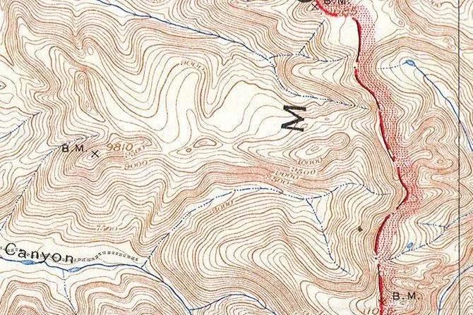
"Teton Range crest (detail), from Grand Teton Quadrangle, Wyoming, USGS topographic sheet, 1929 printing" by U.S. Geological Survey — https://commons.wikimedia.org/wiki/File:1929_U.S.G.S._Map_of_Grand_Teton_National_Park,_Wyoming_-_Geographicus_-_GrandTeton-USGS-1929.jpg — Public domain (US: U.S. Government work (17 U.S.C. §105), USGS topographic sheet surveyed 1899 and first published 1901, this printing 1929 with National Park Service additions; EU: published by U.S. federal agencies more than 70 years ago); modified: cropped, rotated
Contours & Charts
Shaded Relief: Why Maps Light Mountains From the Northwest
Image credit
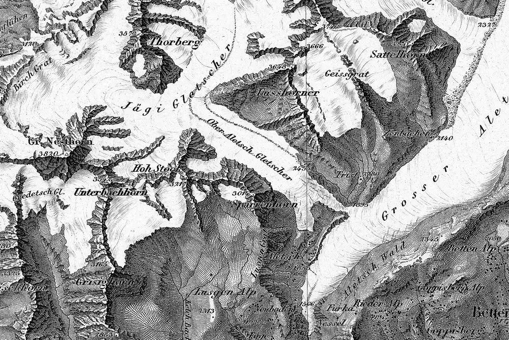
"Blatt XVIII, Brieg, Airolo (detail around the Aletsch glaciers), from Topographische Karte der Schweiz (Dufour Map), 1854, by Guillaume-Henri Dufour and the Eidgenössisches Topographisches Bureau" by Federal Office of Topography swisstopo — https://commons.wikimedia.org/wiki/File:Swisstopo_Dufourkarte_BLATT_XVIII_BRIEG_AIROLO_LT_TK_018_1854.tiff — swisstopo terms of use for free geodata (https://www.swisstopo.admin.ch/en/terms-of-use-free-geodata-and-geoservices); modified: cropped, resized; rights notice: ©swisstopo
Contours & Charts
California as an Island: A Map Error Preserved in Print
Image credit
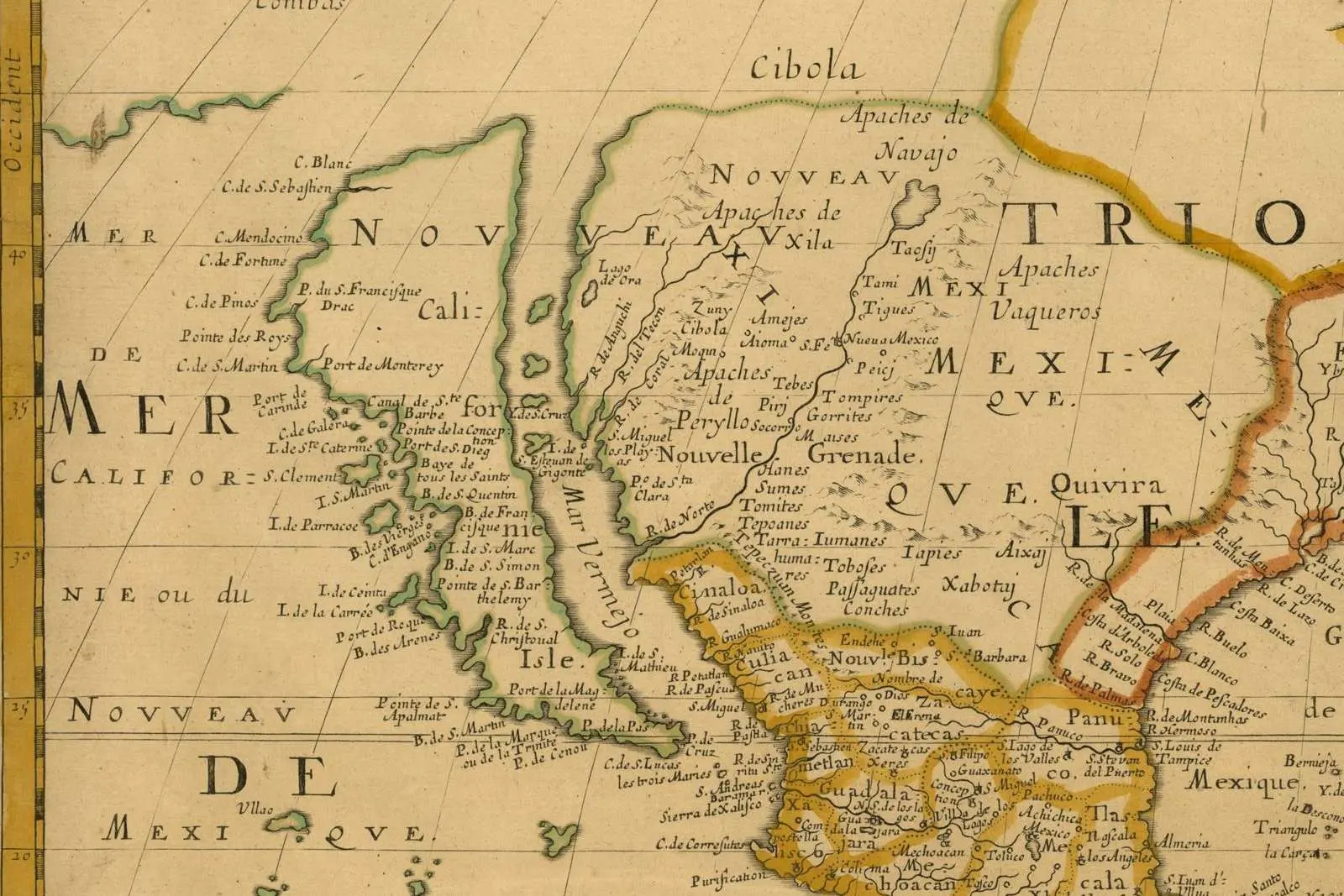
"Amerique Septentrionale (detail: California and the Mar Vermejo), map by Nicolas Sanson, Paris, 1650" by Nicolas Sanson — https://commons.wikimedia.org/wiki/File:Sanson_Amerique_Septentrionale_1650_UTA.jpg — Public domain (US: first published 1650, before 1931; EU: mapmaker Nicolas Sanson died 1667, more than 70 years ago); modified: cropped, resized