How to Read a Geologic Map: A Contact Bends With the Land
The Reading Room Published
Short answer
Put a finger where two colors meet: on a geologic map, that line is a contact between rock units or a fault. The U.S. symbol standard calls such lines a geologic map’s most basic elements.
Viewing card
- Where
- Two maps: an excerpt of the USGS geologic map of the Castle Rock quadrangle, Arizona, and William Smith's 1815 map of England and Wales (map titles as given by the sources)
- Seen from
- From above, as a printed sheet: colored areas, lines and point symbols drawn on a base map (FGDC introductory text, section 3.1)
- Captured
- Smith map dated 1815 (British Library copy); USGS excerpt about 2019; symbols per FGDC-STD-013-2006 (dates of the maps and the standard, not of the rocks)
- Reading altitude
- On paper: about 2 square millimeters is the smallest map-unit area that can show a color; smaller units need a label (FGDC introductory text, section 5.1.3; a guideline, not a fixed limit)
- Written by
- Geologists trace where contacts, faults and folds meet the ground surface and plot those traces as lines on a base map (FGDC introductory text, section 3.4)
This card as data (CSV) About this file
Data: FGDC Digital Cartographic Standard for Geologic Map Symbolization, U.S. Geological Survey Techniques and Methods 11-A2 (2006), public domain, retrieved 2026-11-16
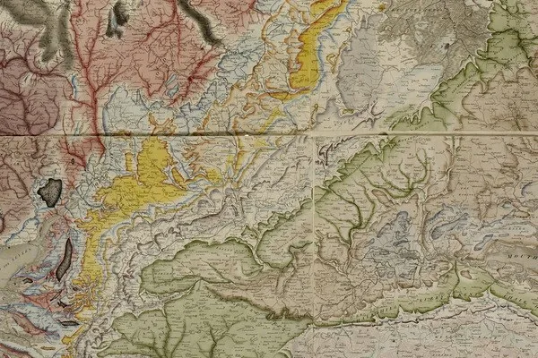
Detail of William Smith’s 1815 map of England and Wales, British Library copy: the colored bands trace the courses of strata where they reach the surface, as Smith described his map in 1816.
"A Delineation of the Strata of England and Wales, with part of Scotland (detail)" by William Smith (1769–1839); British Library — https://commons.wikimedia.org/wiki/File:Geological_map_-_William_Smith,_1815_-_BL.jpg — CC0 1.0 (https://creativecommons.org/publicdomain/zero/1.0/); modified: cropped
The colors on a geologic map are easy to notice and hard to read on their own. Each patch of color stands for a rock unit, and its edges set its shape. A U.S. symbol standard published in 2006 as USGS Techniques and Methods 11-A2 explains why those edges matter. A contact that meets the ground leaves a trace, and once plotted, these traces “become the most basic and fundamental elements of a typical geologic map” (section 3.4).
That standard, the FGDC Digital Cartographic Standard for Geologic Map Symbolization adopted by the Federal Geographic Data Committee, applies to geologic maps published by U.S. federal agencies and their collaborators, and it is the reference for every symbol on this page. The reading below runs in five steps, each with its own section.
- Read the legend. Match each color and label to a rock unit and its age.
- Find the contacts. Trace the thin lines where two colors meet and note whether they are solid, dashed or dotted.
- Find the faults. Look for heavier lines that cut across contacts and offset them.
- Read the tilt. Find the strike and dip symbols and note which way the short ticks point.
- Compare with the contours. Watch how contacts bend where they cross valleys and ridges.
What does a geologic map show?
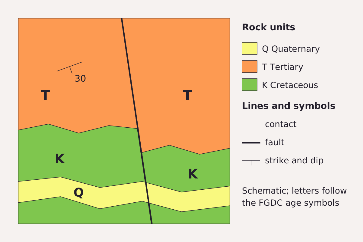
The parts of a geologic map in one schematic: three rock units colored and lettered by age, thin contacts between them, a fault that shifts the contact where it crosses, and a strike and dip symbol.
Benchmark Schematic, not to scale; unit letters and symbols drawn after FGDC TM 11-A2 (2006), Appendix A sections 1, 2, 6 and 32.
"Parts of a geologic map, schematic" by Meridian & Moraine, https://meridianandmoraine.com/strata/how-to-read-a-geologic-map/, licensed under CC BY 4.0 (https://creativecommons.org/licenses/by/4.0/).
Data: Symbols and age letters after FGDC Digital Cartographic Standard for Geologic Map Symbolization, U.S. Geological Survey Techniques and Methods 11-A2 (2006), public domain, retrieved 2026-11-16
The FGDC standard defines a geologic map as “a two-dimensional representation of real-world, three-dimensional geologic features” (section 3.1), and it builds that picture from three kinds of marks. Areas show geologic units, lines trace contacts, faults and folds, and points mark single observations, such as the tilt of a bed or the place where a sample was taken.
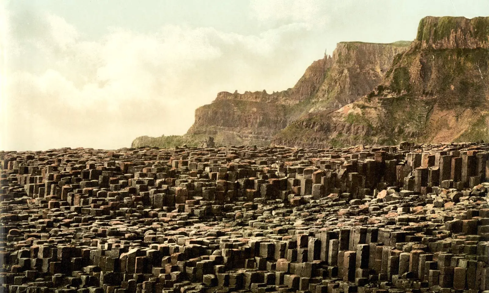
A map unit is a volume of rock whose members share enough traits, such as composition, age or origin, to be treated as a single entity (section 3.3). The standard names the formation as the unit most commonly shown, drawn as an area filled with a color or a pattern, and numbered subunits within a unit can mark individual lava flows (section 3.3.2). The columnar basalt page shows what one flow can look like at the coast.
A contact is the surface that bounds a unit, where the rock changes from one kind to another (section 3.4.1). A fault is a different kind of line, which the standard describes as “a planar surface of rupture along which geologic units have been fractured and then displaced” (section 3.4.3). Because a fault breaks rock that already existed, the standard does not call it a contact, even where it separates two colors.
In the schematic above, the fault is the line where the boundary between the green and orange units suddenly jumps. On the left side of the fault, the contact runs higher on the page than on the right. That offset is the clue that the rock moved after the contact formed.
A geologic map is usually drawn on a base map that also shows the topography, drainage and cultural features of an area, so the geology can be read against the shape of the land (section 3.1). In the United States, geologic map products are archived in the National Geologic Map Database, which the USGS administers (section 1.3). National geological surveys in other countries keep their own map series.
Colors, symbols and the legend
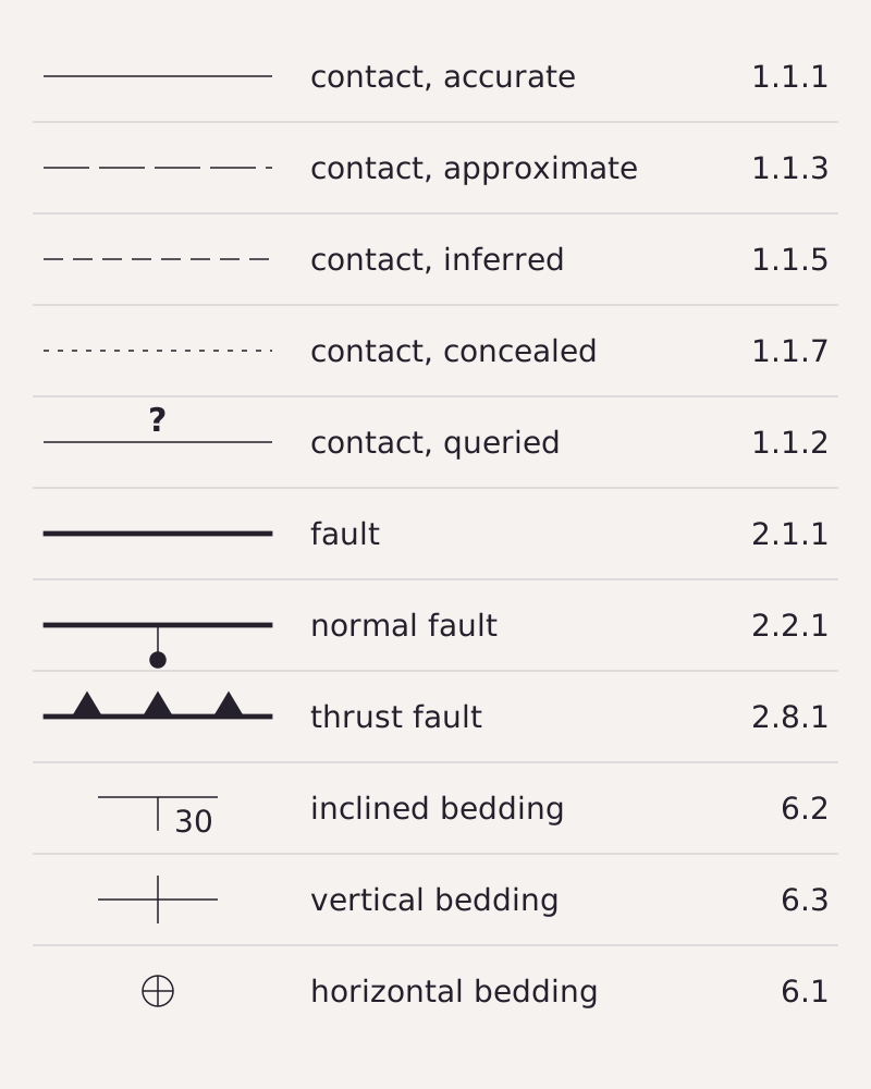
Eleven common symbols from the FGDC standard: four line styles for contacts, a queried contact, three kinds of faults and three bedding symbols, each with its section number in Appendix A.
Benchmark Schematic chart; symbols and section numbers from FGDC TM 11-A2 (2006), Appendix A; each row matches the table below and this page’s CSV.
"Geologic map symbols after FGDC TM 11-A2" by Meridian & Moraine, https://meridianandmoraine.com/strata/how-to-read-a-geologic-map/, licensed under CC BY 4.0 (https://creativecommons.org/licenses/by/4.0/).
Data: Symbols and section numbers from FGDC Digital Cartographic Standard for Geologic Map Symbolization, U.S. Geological Survey Techniques and Methods 11-A2 (2006), public domain, retrieved 2026-11-16
Start with the legend, which lists every unit with its color and a short label. According to the FGDC standard, a label usually begins with capital letters or special age symbols that give the unit’s age, followed by lowercase letters for its name or rock type (section 3.3.2). In the standard’s age symbols, Q stands for Quaternary, T for Tertiary and K for Cretaceous (Appendix A, section 32).
The colors follow a scheme too. The standard says that on geologic maps “color is primarily determined by age and type of rock” (section 5.1.1). Some rock types keep traditional colors: limestone is usually shown in bright blue, glacial till often in light green, and serpentinite and other ultramafic rocks in purple (section 5.1.2). On surficial maps, which show the loose deposits at the surface, color may instead group glacial, landslide, lake and river deposits.
The lines carry a second code. In the standard, a contact is drawn 0.15 mm wide and a fault 0.375 mm wide, which makes the fault two and a half times heavier (Appendix A, 1.1.1 and 2.1.1). Small marks along a fault tell its type: a ball and bar sits on the block that moved down, and sawteeth sit on the upper plate of a thrust fault.
| Symbol | Meaning | FGDC section |
|---|---|---|
| Thin solid line | Contact, location accurate | 1.1.1 |
| Thin long-dashed line | Contact, location approximate | 1.1.3 |
| Thin short-dashed line | Contact, location inferred | 1.1.5 |
| Thin dotted line | Contact, location concealed | 1.1.7 |
| Line with question marks | Contact, identity or existence questionable | 1.1.2 |
| Heavy solid line | Fault, location accurate | 2.1.1 |
| Heavy line with ball and bar | Normal fault; ball and bar on the downthrown block | 2.2.1 |
| Heavy line with sawteeth | Thrust fault; sawteeth on the upper plate | 2.8.1 |
| Long line, short tick and a number | Inclined bedding, strike and dip | 6.2 |
| Long line with two short ticks | Vertical bedding | 6.3 |
| Small circle symbol | Horizontal bedding | 6.1 |
Download the geologic map symbols table (CSV) (about this file) Data: FGDC Digital Cartographic Standard for Geologic Map Symbolization, U.S. Geological Survey Techniques and Methods 11-A2 (2006), public domain, retrieved 2026-11-16
Any single map can bend these rules, because the standard itself says an existing symbol may need to be modified, or a new one created, to fit local geology (section 1.1). When the legend of a particular map and a general chart like this one disagree, the legend is the one to follow.
Following a contact across the map

Open the image full size · annotation layer (SVG)
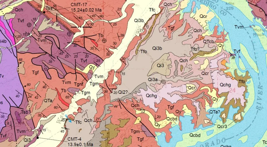
Part of the USGS geologic map of the Castle Rock quadrangle, Arizona, with the Colorado River at the right: three circled features, a thin contact between a pale yellow unit and a purple one, a heavier black line drawn at fault weight, and an inclined bedding symbol marked 50.
Benchmark Schematic annotation layer at the same 900 × 495 px crop as the map; features named from FGDC TM 11-A2 line weights and symbols, not from this map’s own legend.
Image
"Earth MRI geologic map of the Castle Rock quadrangle, AZ (detail)" by U.S. Geological Survey, Earth Mapping Resources Initiative (Earth MRI) — https://www.usgs.gov/media/images/earth-mri-geologic-map-castle-rock-quadrangle-az — Public domain (US: U.S. Government work (17 U.S.C. §105); the usgs.gov media page states Sources/Usage: Public Domain; EU: released by the U.S. Geological Survey with no copyright restrictions); modified: cropped
Annotation layer
"Annotation layer for the Castle Rock quadrangle excerpt" by Meridian & Moraine, https://meridianandmoraine.com/strata/how-to-read-a-geologic-map/, licensed under CC BY 4.0 (https://creativecommons.org/licenses/by/4.0/).
Data: Feature names after FGDC Digital Cartographic Standard for Geologic Map Symbolization, U.S. Geological Survey Techniques and Methods 11-A2 (2006), public domain, retrieved 2026-11-16
This excerpt comes from a geologic map of the Castle Rock quadrangle in Arizona, published on the USGS website under the Earth Mapping Resources Initiative. Its legend is not shown here, so the reading below stays with what the FGDC symbols say. The circled thin line is a contact, and if you trace it with a finger it wraps around the small pale yellow patch.
The circled heavy black line on the left is drawn at the weight the standard gives to faults. It runs nearly straight down the excerpt while the thinner contacts around it bend. The small arrow on it, marked 60, sits where the standard places a dip reading taken on a fault line (section 3.6.1.1), but only the map’s own legend can say what it records.
The style of a line tells how well its position is known (section 4.2.4). A solid line means the feature can be seen in outcrop and is plotted within the map’s stated accuracy, while a long-dashed line means it was seen but could not be plotted as precisely. A short-dashed line means it was hidden under deposits, debris or plants and was estimated between a few outcrops, and a dotted line means it is buried under another mapped unit or under water or ice.
Every geologic map also simplifies. The FGDC standard puts the smallest area that can show a color at about 2 square millimeters on the printed map, and the smallest area that can show a pattern at about 1 square centimeter, so a smaller unit needs a label (section 5.1.3). Scale changes the lines too: a contact that is gradational on a 1:24,000 map “would probably be considered discrete at a scale of 1:100,000” (section 3.4.1.1).
That loss is the cartographer’s cut on a geologic map: the pieces of rock too small to color, and the transition zones flattened into a single line. What the sheet shows is a drawing of the rock at one scale, not the rock itself.
Strike and dip: which way the layers tilt
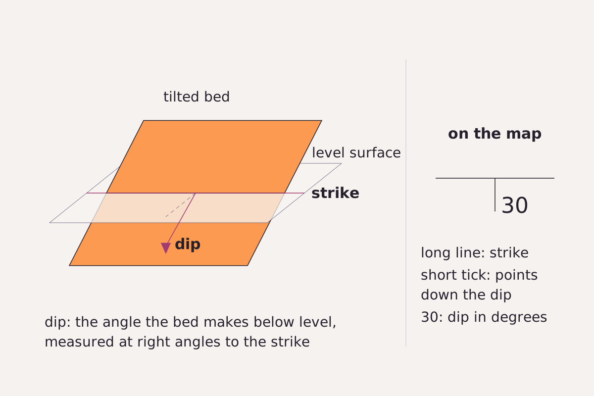
A tilted bed meets a level surface along its strike; the dip is the angle the bed makes below level, and the map symbol on the right carries both.
Benchmark Schematic, not to scale; definitions and symbol from FGDC TM 11-A2 (2006), section 3.6.1 and Appendix A, section 6.
"Strike and dip of a tilted bed, schematic" by Meridian & Moraine, https://meridianandmoraine.com/strata/how-to-read-a-geologic-map/, licensed under CC BY 4.0 (https://creativecommons.org/licenses/by/4.0/).
Data: Definitions and symbol from FGDC Digital Cartographic Standard for Geologic Map Symbolization, U.S. Geological Survey Techniques and Methods 11-A2 (2006), public domain, retrieved 2026-11-16
Two measurements fix the tilt of any planar surface, such as a bedding layer or a fault plane. The FGDC standard defines the strike as the direction of the line where the surface meets an imaginary level surface. The dip is “the angle of departure of that surface downward from horizontal, as measured perpendicular to the line of strike” (section 3.6.1).
On the map, the symbol has a long shaft along the strike and a short tick that points down the dip, with the dip angle written beside it as a number (section 3.6.1.1). The point where the shaft and the tick meet marks where the measurement was taken. A vertical bed gets two ticks, one on each side, and a flat bed gets a symbol with no direction at all.
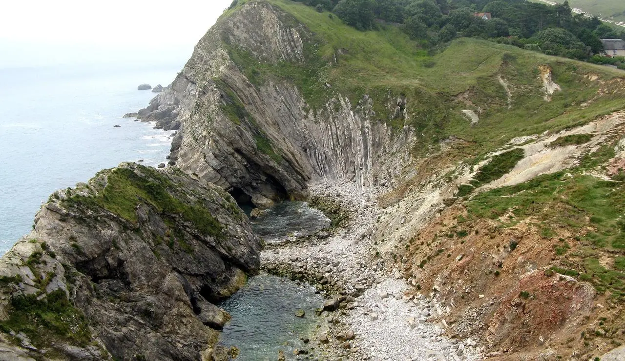
The circled symbol marked 50 on the Castle Rock excerpt has the shape of the inclined bedding symbol, so, if the map follows the standard, it records layers tilted 50 degrees below level in the direction of its tick. Nearby symbols carry other numbers, such as 30, 25 and 20, so the recorded dips differ across a short distance. Where layers are warped, the standard calls the structure a fold (section 3.4.4), and the Lulworth Crumple page shows one in a coastal rock face.
The standard also has special symbols for beds whose top direction is known from features in the rock, and for beds that are overturned (Appendix A, section 6). Those are worth looking up in a map’s legend before reading the tilt of strongly folded rocks.
When a contact crosses a valley
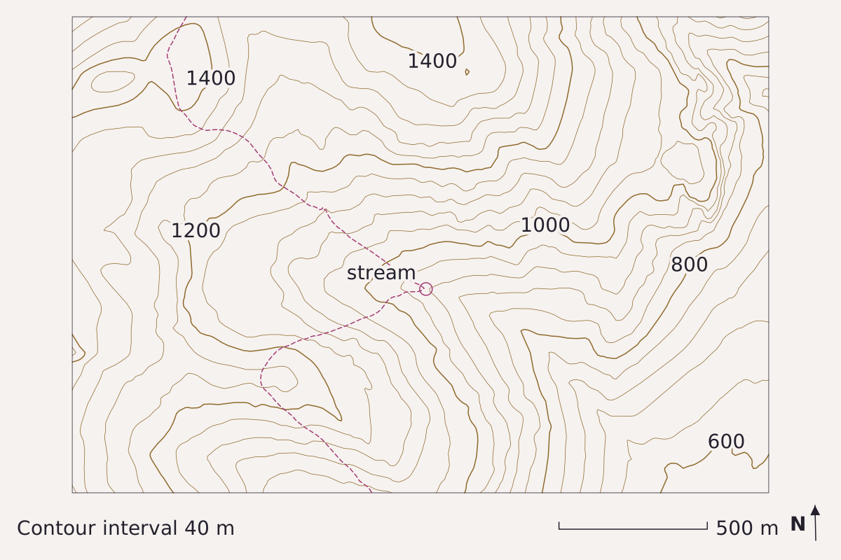
Real ground, imagined rock: the dashed line is where a flat contact dipping 30° to the east would meet the land in the elevation model. In the valley the contours point upstream, to the west, but the contact’s trace points downstream, to the east, because the layer dips downstream more steeply than the stream bed falls (about 20° here). North is up, with the map grid about 1.2° off true north. Elevation: USGS 3DEP 1/3 arc-second, n48w122 2025-08-13.
Benchmark Contours from USGS 3DEP 1/3 arc-second DEM; interval 40 m; 5 points checked against the DEM; map corners recomputed from the DEM's georeferencing.
"When a contact crosses a valley" by Meridian & Moraine, https://meridianandmoraine.com/strata/how-to-read-a-geologic-map/, licensed under CC BY 4.0 (https://creativecommons.org/licenses/by/4.0/).
Data: Data available from U.S. Geological Survey, National Geospatial Program.
A contact on a map is a line, but the contact itself is a surface. Where that surface meets uneven ground, its trace bends with the land. The map above tests this with a real valley in the Cascade Range of Washington, drawn from the USGS 3DEP elevation model, and an imagined contact.
The contact is a flat plane tilted 30° toward the east, set to pass through the valley floor at an elevation of 923 m, and the dashed line traces where that plane meets the ground. On the contour lines page, the contours of this same valley bend into a V that points upstream. The contact trace here bends the other way.
In this model, the reason is a race between two slopes. Near the crossing, the elevation model has the stream bed dropping about 115 m over about 310 m, a slope of about 20°, while the layer dips at 30° in the same direction. Because the layer drops faster than the bed, it reaches the valley floor farther downstream than it reaches the valley sides, and its trace points downstream.
The figure has its own cartographer’s cut. The contact is a perfectly flat plane, which real contacts are not, and the 40 m contour interval hides the small side gullies where the trace would bend again. The five points in the CSV below compare the contours with the elevation model, not with any mapped geology.
Download the elevation comparison points (CSV) (about this file) Data: Data available from U.S. Geological Survey, National Geospatial Program.
William Smith’s 1815 map
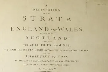
The title block of William Smith’s 1815 map: “A Delineation of the Strata of England and Wales, with part of Scotland,” with the collieries, the fen lands and the varieties of soil named below.
"A Delineation of the Strata of England and Wales, with part of Scotland (title block)" by William Smith (1769–1839); British Library — https://commons.wikimedia.org/wiki/File:Geological_map_-_William_Smith,_1815_-_BL.jpg — CC0 1.0 (https://creativecommons.org/publicdomain/zero/1.0/); modified: cropped
William Smith’s map of England and Wales, dated 1815, colors the land by its strata in long bands that run from the south coast toward the northeast. On the British Library copy shown here, the bands change color where one set of strata gives way to the next, much as the colors on the Castle Rock excerpt do.
Smith explained what the map recorded a year later, in the introduction to Strata Identified by Organized Fossils (1816). He wrote of “thus distinguishing so great a variety of materials in the earth, as successively terminate at the surface,” and of “their courses delineated in a large map of the Strata just published.” Read plainly, the colored bands mark the places where each stratum reaches the ground.
The same page says how Smith told the layers apart. Smith wrote that his attention was drawn to fossils “by a previous discovery of regularity in the direction and dip of the various Strata in the hills around Bath,” words that describe the same kind of tilt a modern strike and dip symbol records. The paragraph then introduces his account of the “organized Fossils” found in each stratum, the clue the book’s title refers to.
A map like this can be read as a page of rock manuscript laid flat, with each band one line of text. Every color edge on Smith’s map marks where, by his reading, one rock layer stops at the surface and another starts. Like the maps of California as an island, an old map such as this records what its maker knew at the time, and its lines can be compared with later surveys.
Next time a geologic map is open in front of you, skip the colors at first. Put a finger on one contact and follow it until it meets a fault, a valley or the margin of the sheet, then check the legend to see which two units it separates. Finally, look for the nearest strike and dip symbol to see which way those units tilt.
Next overpass
- Siccar Point: stand the map up on edge, and one contact on a sea cliff records at least four events.
- Richat Structure: a dome worn flat shows its layers as rings, like color bands on a map seen from orbit.
Sources
- Federal Geographic Data Committee, FGDC Digital Cartographic Standard for Geologic Map Symbolization (PostScript Implementation), prepared by the U.S. Geological Survey, U.S. Geological Survey Techniques and Methods 11-A2 (FGDC-STD-013-2006), 2006. pubs.usgs.gov/tm/2006/11A02/Read: full text of the introductory text; Appendix A sections 1 (contacts), 2 (faults), 6 (bedding) and 32 (geologic age symbols)
- U.S. Geological Survey, Earth Mapping Resources Initiative (Earth MRI), “Earth MRI Geologic map of the Castle Rock quadrangle AZ,” USGS media image, about 2019. www.usgs.gov/media/images/earth-mri-geologic-m…Read: page (usgs.gov media page) and the full-width image; the map's legend and report not read
- William Smith, Strata Identified by Organized Fossils, Containing Prints on Colored Paper of the Most Characteristic Specimens in Each Stratum (London, 1816). archive.org/details/Strataidentifie00SmitRead: pages 1–2 of the Introduction (unnumbered), checked against the page images
- William Smith, A Delineation of the Strata of England and Wales, with Part of Scotland (London, 1815); British Library copy, digitized by the British Library. commons.wikimedia.org/wiki/File:Geological_map_-_Willia…Read: file page and the full map image (title block and colored bands examined)
- U.S. Geological Survey, 3D Elevation Program 1/3 arc-second Digital Elevation Model, tile n48w122 (USGS 1/3 Arc Second n48w122 20250813, publication date 2025-08-13), The National Map. prd-tnm.s3.amazonaws.com/StagedProducts/Elevation/13/TIFF/…Read: values: elevation grid windows 47.7725–47.7975° N, 121.365–121.315° W (33-0003); 47.75–47.83° N, 121.27–121.41° W (33-0011); 47.7725–47.7875° N, 121.350–121.318° W (33-0012)

Cite this page
The Reading Room. “How to Read a Geologic Map: A Contact Bends With the Land.” Meridian & Moraine, published 16 November 2026. https://meridianandmoraine.com/strata/how-to-read-a-geologic-map/. Accessed on the date you read it.
How readings are checkedAll correctionsReport an error on this page (contact@meridianandmoraine.com)
More from Reading Rock Layers
Reading Rock Layers
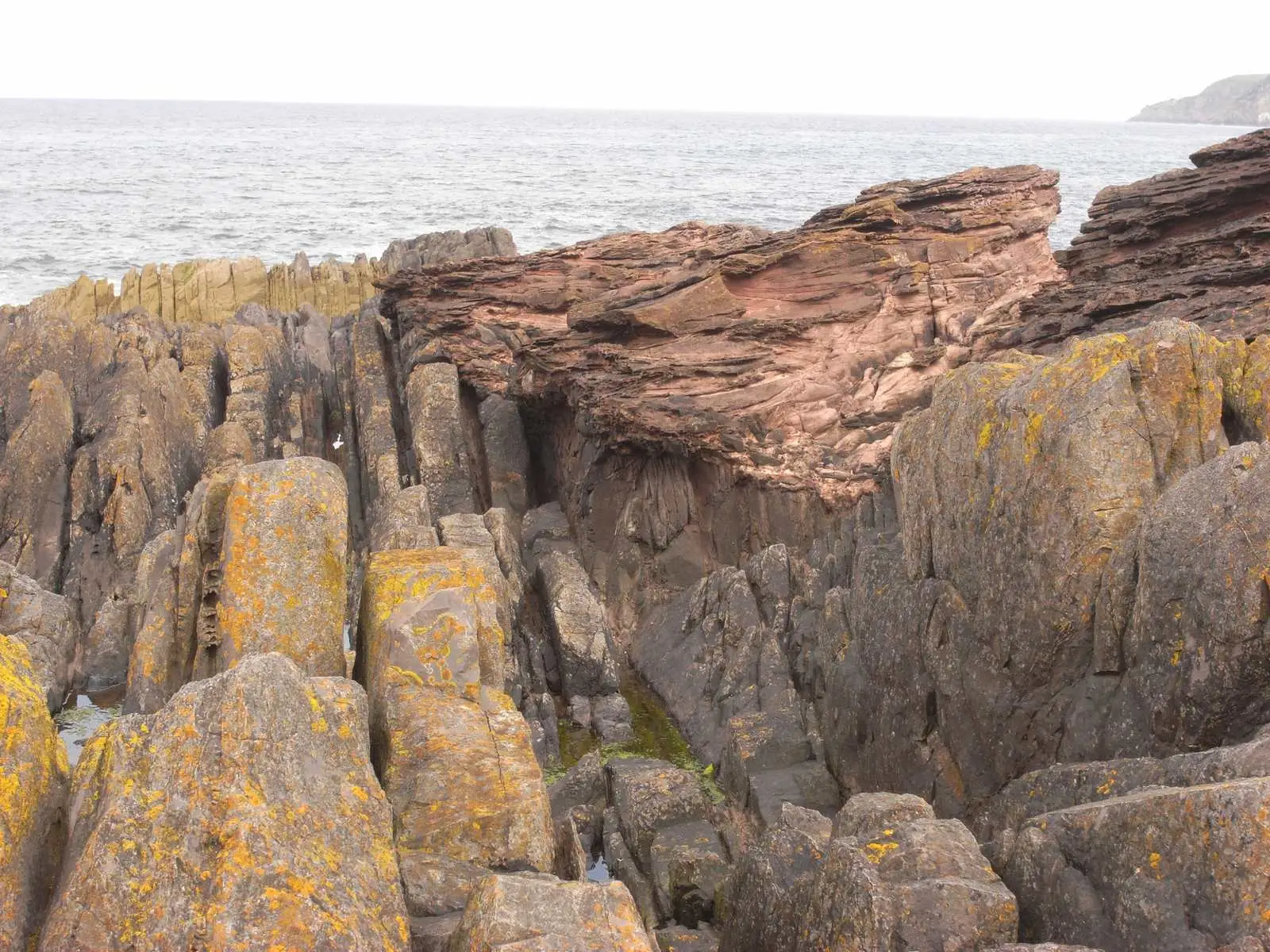
Siccar Point: Hutton’s Lower Beds Stand Almost on End
Image credit
"Hutton’s Unconformity at Siccar Point, Scotland" by Lysippos — https://commons.wikimedia.org/wiki/File:Hutton%27s_unconformity_siccar_point.JPG — CC BY 3.0 (https://creativecommons.org/licenses/by/3.0/); modified: resized
Reading Rock Layers
Lulworth Crumple: The Limestone Cracked, the Mudstone Flowed
Image credit
"West end of Stair Hole, Lulworth, Dorset, England" by Adrian Pingstone — https://commons.wikimedia.org/wiki/File:West_end_of_Stair_Hole,_Dorset,_England_arp.jpg — Public domain (US and EU: released into the public domain worldwide by the photographer, Adrian Pingstone, as stated on the Commons file page); modified: cropped, resized
Reading Rock Layers
Columnar Basalt: Not Every Causeway Column Is a Hexagon
Image credit
"Giant's Causeway, County Antrim, Ireland, photochrom published by the Detroit Publishing Co. under license from Photoglob Zürich" by Unknown author — https://commons.wikimedia.org/wiki/File:Giant%27s_Causeway,_County_Antrim,_Ireland,_1890s.jpg — Public domain (US: published before 1931 (photochrom printed between 1890 and 1900); EU: anonymous work, photographer not named, first published more than 70 years ago); modified: cropped, resized